 It’s third down and one yard to go. Should the coach call for a run or pass? We know that according to game theory (and from simple experience), it’s best for a coach to call for a randomized mix. The question is, what is the optimum mix? In other words, what are the best run/pass ratios in 3rd down situations? We’ll see if coaches are making the right calls on 3rd down, focusing on 3rd and 1 as a case in point.
Game theory tells us that, at the optimum mix of strategies, the average utility of both strategies will be equal. The optimum mix of strategies is also known as the Nash equilibrium. In football terms, that means that on 3rd and 1 yard to go, if a team is getting a 1st down 60% of the time when running and 30% when passing, that team is passing too frequently.
If this just sounds like theoretical mumbo-jumbo, and you don’t buy that the payoff for running and passing should always be equal at the optimum ratio, think of it this way: If the conversion rate for running is higher than that for passing, why pass at all? The answer is obvious enough—If offenses only ran, defenses would stack the line with all 11 defenders and the success rate would plummet. So the best tactic would be to run more often until defenses counter your tendency. Defenses would be forced to commit to run defense more and more until passing becomes more successful. When the conversion rate for running and for passing equalize, that’s the Nash equilibrium where the overall conversion rate will be highest.
A look at conversion rates across the NFL for 3rd downs at various ‘to go’ distances initially suggests offenses pass too often on 3rd and short. Notice how the conversion rate is higher for running than for passing for short yardage situations.
On 3rd and 1, teams are successful in 70% of attempts when running, but in only 58% of attempts when passing. Not until we get to 3rd down and 5 yards to go do the conversion rates completely equalize.
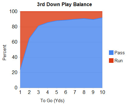
Except for the 3rd and very short situations, I’m struck by how close the conversion rates for running and passing are. Running and passing were equally successful for 3rd down and mid- to long-yardage situations. For example, for the 1011 3rd and 7 situations in the past 8 years, both running and passing were successful 38% of the time. Teams are running in that situation only 12% of the time, so defenses are usually expecting a pass.
Running therefore becomes far easier than if teams ran more often on 3rd and 7. Whether they realize it or not, NFL coaches are doing an excellent job finding the Nash equilibrium, at least on 3rd and 5 or more. The graph below plots the NFL-wide 3rd down run/pass balance for various ‘to go’ distances. Passing is the preferred option at longer distances for obvious reasons.
Converting a 1st down is not, however, the only measure of success. It’s always better to have a 1st down and more yards (except on 3rd and goal). So passing seems to offer an advantage over running because its average gain is longer. On the other hand, passing adds the slight possibility of an interception. I'll examine those considerations in part 2 by comparing the average gain for both play types and by analyzing the expected points scored after run attempts and after pass attempts on 3rd down.
Note: The data are from all regular season 3rd down run and pass plays from 2000 through 2007, except for those within 2 minutes of the end of a half and all plays from within field goal range defined as inside the 35 yard line. I excluded late minute plays to exclude situations where teams were tending towards the pass for clock management purposes. Plays within FG range could skew the results because teams may make non-optimum decisions knowing they can kick a FG if unsuccessful. Conversion rates include 1st downs due to penalties. One shortcoming in the data is that QB scrambles are counted simply as runs. However, scrambles comprise a very small minority of plays, so the general conclusions here should not be affected.
Play Calling on 3rd and Short Part 1

Fantasy Football and the Wisdom of Crowds
 On most fantasy football sites, including the one my league uses—Yahoo, team owners can see which players are the most popular. When you’re drafting you can see in which round other leagues have taken each player. And during the season you can see how many other teams feature each player as a starter or on a roster.
Personally, I never paid much attention to the preferences of the drooling slob masses of football fandom. I figured I was a little sharper than the average fan, so why pay attention to shirtless people wearing wear purple camouflage pants and team-logo emblazoned construction helmets with integrated beer dispensers?
But I was wrong. And here’s why.
I have biases. Being from Baltimore, I like the Ravens, and I have a burning hatred for the Colts. For years I would never pick a Colt for my fantasy team, even passing over Peyton Manning for Daunte Culpepper in the 1st round in 2005. (6 TDs. Ouch.) I'm sure many Cleveland fans feel the same way about Baltimore.
I also make plain old errors and misjudgments. I very often miscalculate how well a player will do or his likelihood of injury. I’m wrong far more often than right. Every one of my opinions has biases and errors. We all have biased and incorrect opinions. You do, and so does that guy, and that other guy over there. We all have them, some more than others.
So if you combine everyone’s opinions, you’d think we’d end up with nothing but a jumbled sea of moronic idiocy. But we don’t. We usually get a very accurate estimate of the truth. Averaging a large crowd’s opinion can be so accurate because our biases and errors usually don’t add up. They cancel out. Let’s take some target practice. A thousand people who have never shot a gun before go to the range and each fire once at a target downrange. There would be very few bullseyes that day. But if we averaged out everyone’s error, we’d likely come very, very close to a bullseye for the group.
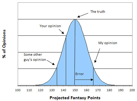
Now, instead of target practice, let's try to estimate Marion Barber's fantasy production this year. I think the best guess is that he'll have about 167 total points this season. You're a little smarter than me, and you know he's carrying the whole load in Dallas this year, so he might wear down or get injured. You guess 142 points. Some other guy doesn't know anything and he hates the Cowboys so he's got Barber pegged with 133 points. None of us are right, but all of us together are going to be pretty close.
I'm not claiming that collectively we can predict exactly how Marion Barber will do this year. I'm suggesting that together, our collective judgment will be a lot closer to the best unbiased estimate possible than any individual guess, even by 'experts.' After all, Barber could be out for the season on his first carry this year, but that doesn't make our best estimate wrong.
The weakness of the wisdom of crowds concept is when there is a systematic bias in everyone's opinion. In our target practice analogy, the barrel of our gun is warped. This can most often occur from media hype, or when one or a few very influential experts shape our opinions--think Mel Kiper. But when opinions are formed independently, or when there isn't a small group of dominant experts, biases and errors tend to be random. And when there are random errors, the larger the sample, the better the result. That's why I trust the fantasy football crowd.
Fantasy football is largely an internet phenomenon, and there doesn't seem to be a Mel Kiper of fantasy, but lots of expert-wannabees instead. It seems most fans know these experts are mostly turkeys, and make their own opinions in relative isolation. So I tend to believe the crowd, morons and all, more than my own judgment.
There's actually a book out now on this phenomenon. I haven't read it yet, but it's nearing the top of my list. Check out The Wisdom of Crowds by James Surowieki if you're interested.
Game Theory and Fantasy Draft Strategy
 My last article (part 1, part 2) took a look at the concepts at the core of fantasy draft strategy. Scarcity and consistency are, in my opinion, the critical considerations when valuing players. I also outlined an 'opportunity cost' concept in player selection. In this article, I'll take a look at particular draft strategies and try to push the envelope a couple inches.
Replacement-Level Strategy
For those not familiar with replacement-level drafting strategy, it's based on the relative value of each player above the lowest ranked player within each position. But before you do anything, you need some sort of value assignment for each player, the most logical being their total projected fantasy point production. You can use anyone's projections, such as Yahoo's, or FFToolbox, or any of the array of websites that offer them. You can just as easily use your own, or modify a published list. It (almost) goes without saying that you need to make sure the scoring rules used for the values are the same as those for your league.
If your league starts 1 QB, 2 RB, 3WR, and a TE, and your league has 8 teams, the replacement level player at each position would be the 8th-ranked QB, the 16th-ranked RB, the 24th-ranked WR, and 8th-ranked TE. For example, using my office league's scoring rules, LaDanian Tomlinson is projected by Yahoo to produce 224 points, and the 16th ranked RB is Selvin Young who is expected to produce 117 points. This gives LT a 224 - 117 = 107 value over replacement player (VORP).
Before your draft, you would calculate the VORP for each player, and simply draft the player with the highest value until each starting roster slot is full. This is also known as value based drafting (VBD). I like this system. It's simple and it usually works very well. However, it fails to fully capitalize on the irrationality of your opponents.
Implications from Game Theory
A fantasy football draft, or any similar draft including the NFL's actual draft, is what game theorists would call an n-player zero-sum game with perfect information. N-player means more than 2, which severely complicates any analysis. It's a zero-sum game because there is a finite amount of projected value available to the entire league, and players are scrapping for the largest share. (Players can voluntarily make non-optimum choices, and so the game could be considered non-zero-sum, but game theory always starts with the assumption of rational players.) Perfect information refers to the fact that you are aware of every move made by other players up to the current point in the game.
N-player games cannot be 'solved' the same way as 2-player games can, as I demonstrated with the example of the run-pass balance problem. But in game theory, there is usually a 'minimax' solution to zero-sum games. Also known as a Nash equilibrium, the minimax solution is the strategy with the maximum assured minimum gain for a player. (Technically, it's the strategy that minimizes the opponent's maximum possible score, which is effectively the same for a zero-sum game.)
Although it's technically imprecise to call it so, the VORP strategy is akin to a minimax for a fantasy draft. It guarantees you a minimally assured value total for your starters. But like all minimax strategies, it can be extremely conservative because it assumes other players are purely rational and also play their minimax strategy.
But in many cases, most other fantasy opponents are not playing a VORP strategy. They'll be biased towards hometown favorites, or picking based on hunches, or simply following a rule of thumb such as RB-RB-QB-WR... (like I typically do). They'll leave better players on the draft board than would otherwise be there. However, chances are that other opponents will be there in front of you to snatch them first. Fortunately, there is another, slightly more aggressive approach that can get even more points.
Value Over Next Available
If you have a good idea, or any idea, about what positions will come off the board between your own picks, you can adjust your choices to capitalize on your opponents' errors while maximizing your projected values beyond the minimax. You can get a reasonable estimate of how many QBs, RBs, etc will be taken in each round in several ways. First, guys talk football draft strategy like women talk about clothes. Every guy thinks he's smartest football expert in the room. (Gosh, I hate guys like that...) If your opponents haven't blabbed their first couple picks, then it doesn't take a CIA ops officer to get them to spill the beans. But a more reliable method might be to just look at mock drafts and historical trends. For example, I found that for an 8-team league in '08, the expert mock drafts I clicked on last night typically looked like this:
1st round: 1 QB, 7 RBs
2nd round: 5 RBs, 3 WRs
3rd round: 3 RBs, 1 QB, 4 WRs
Plus, as the draft goes on, you can refine the estimates based on which players have already been taken. Team A still needs a QB...Team B took a WR in round 1, he'll need a RB...etc. That's where the "perfect information" comes into play.
As your pick approaches, estimate the number of each position that will be taken between that pick and your subsequent pick. For example, in my recent 8-team league draft, between my 4th pick in the 1st rd and my 13th overall pick in the 2nd round, I estimated there would be 1 QB, 2 WR, and 5 RBs taken. (Before my 1st pick there was 1 QB, 1 WR, and 1 RB taken.) I calculated the difference between the best available RB and the RB 6 spots down the board, because he's the next RB available to me if I don't take a RB this round. I also calculated the difference in value between the best QB available, and the next best QB. Finally, I calculated the difference between the best WR available and the WR 2 spots down the board. These differences are the costs of not picking each position in that round. I picked the position with the highest cost. Instead of my usual RB-RB-QB-WR... pattern, this system had me pick RB, WR, QB, TE(!), RB, WR, WR. I ended up with 950 projected points. The next highest team had 850. The next highest opponents essentially used a VORP method and ended up with 815 and 814. Using my conventional strategy in an earlier dry run with the same opponents using the same strategies, I got only 694 pts, 5th out of 8 teams. One draft does not prove the system, but it does have a solid theoretical underpinning.
For those interested, I've set up a spreadsheet with an example draft that demonstrates the system, which has been dubbed VONA for Value Over Next Available. Each round of my mock draft has its own tab at the bottom of the spreadsheet. There is a text box on each worksheet that explains each selection. I don't think my system is terribly revolutionary, but it is an improvement. It's really just a dynamic VORP system. The difference is that the replacement player at each position changes as the draft evolves. The advantage comes from being able to better capitalize on opponent error.
Some Final Thoughts on Draft Strategy
1. I really like the replacement-level concept. As long as you have an objective value for each player, it will do an excellent job at ensuring a minimum level of success. If you don't have a good idea of how many players at each position would be taken between your own picks, you'll want to stick with VORP. Here a couple additional tricks I thought of:
a. If someone picks a player below your replacement player at a certain position, your replacement player has now changed, and you should adjust your VORP numbers. For example, in a 10-team league, if someone grabs the #11 QB, your replacement player is now the #9 QB. He's now the worst-case scenario at QB for you.
b. Depending on your draft position and how many starting slots your league has, your replacement level players aren't who you think they are. If you have the 10th pick in a 10 team draft, with 6 (or any even number) starting slots, you will pick 1st in the last round. The last 9 players are inconsequential. You can safely eliminate 2 or 3 of the bottom TEs and WRs (and perhaps the 10th QB) from your list. They'll be taken after your last pick (of offensive starters). The same principle applies if you have the 9th pick or 8th pick, or the first few picks with an odd number of starting slots.
2. You may value a backup RB more than a #3 WR, or even a mid-range TE. That's up to you. If you do, just consider the #3 RB as a starting slot, and the VORP or VONA system will still work.
3. We haven't discussed kickers or defenses yet. But everything I've seen says they're the least predictable and most replaceable. Plus, defenses can easily be picked up according to weekly match-ups. Maybe that's something to be looked at in detail in the future.
4. All of this probably doesn't matter.
It's true. The vast majority of decisive factors are luck--injuries, other unforeseeable events, sudden declines of teams, or even weather (Remember the Pats-Jets game in the snow/wind storm last year--it helped get me in the playoffs). If in a 10-team league you have a 10% chance of winning, perfectly optimizing your draft gives you, what, a 12% chance? 13%?
5. Finally, if you win at fantasy football, it doesn't mean you know anything about the NFL or its players. Unless you're an NFL scout, it very probably means you are just lucky. Everyone has access to the same volumes of up-to-the-second information, projections, and match-ups for every NFL player. Even if fantasy football was as much 50% skill, you'd need to compete successfully for several years before you had really any certainty that you were any good.
Now that I've sapped every last drop of fun out of it, enjoy your draft and good luck!
Fantasy Draft Strategy Part 2
 In part 1 of this article, I analyzed the scarcity and consistency of fantasy performance at each position. We saw that picking the best available player is not the best strategy. In the second half of this article, I'll tie those two concepts together and outline a draft strategy that optimizes your expected points from your starters.
Summary and Observations
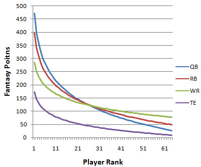
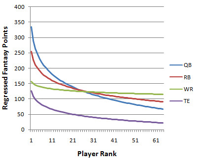
Here is a graph summarizing the drop-off curves for the performance of the offensive fantasy positions. Each position's drop-off is nearly perfectly logarithmic. (Wow--logarithms and fantasy football?)
The graph above only factors in actual performance--it's a picture of scarcity and absolute point totals. It does not consider the different consistency levels of the various positions. The version below regresses the curves according to the consistency of each position, combining the concepts of consistency and scarcity.
Compare the TE curve (purple) and the WR curve (green) in the graph immediately above. At no point does the TE curve exceed the WR curve in absolute terms. But the TE curve is steeper, which indicates that the differences between the top available TE and the next-best-expected TE is greater than that for WRs throughout the draft.
We shouldn't be concerned with the height of the lines, but with their slopes. Because each fantasy team is forced to start a certain number of players at each position, you only need to be concerned with the advantage you have within that position. If your TE is projected to produce 25 more pts over the season than the next best TE, and your WR corps is projected to produce 15 pts less than an opponent, you have a 10 pt overall advantage. It doesn't matter that WRs score twice as many points as TEs.
If everyone knew this, they'd jump on the top few TEs before even picking their first WR (in most years). But they don't, so you can take advantage by waiting to pick a TE until the last round before you think the first TE will be chosen. Just be sure to be the first guy to grab whoever is the Gates/Gonzalez/Witten/Clark of the current year.
Opportunity Cost
The best way to explain this strategy is opportunity cost. Don't pay attention to the overall ranking or projection of a player. Focus within positions. Judge the difference in value between the best player available in each position, and what you think the next best available player will be to you. In essence, calculate the cost of not picking the top available player at each position. The position with the highest cost should be chosen.
Say you have the 5th pick in a 10 team draft, and the previous 4 picks were RBs. You can estimate that between your 5th overall pick in the 1st round and your 16th overall pick in the 2nd round, there will be 8 RBs taken, 1 QB, and 1 WR taken. No TEs will be taken, so you don't even need to worry about them yet. So calculate the cost of not picking a RB, a QB, etc. You should calculate the difference between the #5 RB and the #13 RB, between the #1 and #2 QB, and between the #1 and #2 WR. Whichever difference is greater should be your pick.
Every year will be slightly different, based on the relative projections of the top players at each position. So we can't always say that a particular order of positions is the optimum one. But the 'opportunity cost' strategy will give you the highest possible projected point total for your starters coming out of the draft. It's not guaranteed because it depends on your estimates of how many players at each position will be chosen between your picks. But that isn't too difficult, and it can be updated as the draft goes on. Happy drafting.
Fantasy Draft Strategy
 For most guys, fantasy football drafts bring to mind pitchers of beer and pizza. While I love both those things, I also think about...logarithms. Although I don't focus on fantasy football here, it's hard not to write about NFL statistics without at least one or two fantasy articles each season. Hopefully, this will satisfy some of the email requests I get this time of year.
I play in my office's league each year, but I'm not one of those guys that does lots of research or pays a website for their recommendations. But this year I decided to put some thought into how to have the best draft. Two primary questions came to mind.
First, how consistent are the various elite players at each position? In other words, how reliably do last year's stars repeat as elite players this season? For example, are QBs more consistent than RBs? The more reliably consistent a position is, the more certain we are to get value from spending a high pick on it. Second, how large is the drop-off in performance at various positions? For example, how does the scarcity of good RBs compare to that of WRs? The scarcer the position, the earlier it should be drafted.
Using data from the past five NFL seasons, I'll quantify both the consistency and scarcity of each position, then combine both concepts to make recommendations about fantasy draft strategy.
Consistency and scarcity are the two most important considerations when choosing a player, particularly in the first several rounds. Overall total value is nearly totally meaningless, which means picking the "best available player" is far from the best strategy. I'll illustrate why. And unfortunately, yes. It has to do with logarithms.
Scarcity
Imagine a 5-team league in which the scoring rules project the top 5 QBs to score 400, 395, 380, 375, and 370 points. The top 5 RBs are projected to score 300, 250, 200, 150, and 100 points. Who would you choose with the first pick? The best available player strategy dictates you take the #1 QB, projected to produce 400 points. Your second round pick would likely be the #5 RB at 100 pts, giving you a 2-round total of 500 projected points.
But by considering scarcity, you'd see that the drop-off among RBs is far steeper. Chosing the #1 RB with 300 pts, and the #5 QB with 396 pts, yields a total of 670 projected points. This is an exaggerated hypothetical, but it exemplifies the fallacy of choosing the best player. What really matters is the difference between the top available player and the expected next best available player at each position. That difference is what should dictate your selection.
In the example above, the difference between the top QB available (400) and the next best expected QB available (365) is 30 points. The difference between the top RB available (300) and next best expected RB available (100) is 200. Looking at it terms of next-best-available, the RB is the obvious choice.
Consistency
Let's say that we're deciding between taking a RB and a WR in the 3rd round. Assume the scarcity differences happen to be equal for both positions. Our best expectation is that 4 RBs and 4 WRs will go off the board between our 3rd round pick and 4th round pick. The best available RB is projected to produce 100 pts and the next expected available RB is projected to produce 50, for a difference of 50. The WRs available have the same exact values. How should we decide?
What if top RBs reliably repeated their performance from year to year at an 80% level of consistency, but WRs were up and down from year to year, keeping on average only 60% of their performance levels? We should bank on the RB in the 3rd round, and save the gamble on a WR for a later round.
But, if year-to-year WR performance is highly variable, doesn't that mean they could improve too? Sure, but there's not a lot of room for improvement at the top. Players with the very top performances in one year are far, far more likely to decline, even if slightly, than to improve. Plus, if there is indeed a lot of upside potential in WRs, why not wait until a later round to start grabbing them?
A lot of this might seem obvious to some people, and it's why the typical draft pattern goes RB-RB-QB-WR-WR... So why not quantify these concepts and see if fantasy football conventions hold up?
Quarterbacks QB is a relatively consistent position. The year-to-year correlation in fantasy points for the top 32 QBs the past 5 seasons is 0.60. This means that if we want the best guess as to how many fantasy points to expect, we would use 60% of their difference from the average. So if the average QB gets 100 points in a season, and the QB we're thinking about drafting got 160 last year, for 2008 we should expect:
Regression to the mean gives us our best statistical estimate. It accounts for injuries, natural improvements or declines, change in teammates, change in opponents--everything. We can say QBs are about 60% consistent.
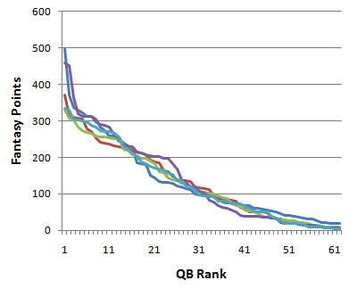
QBs are relatively scarce too. After the top 1 or 2 guys, there is a steep fall-off in performance illustrated by the graph below. (Each line is for one of the past five seasons. 'Rank' refers to actual performance, not order in which players were drafted.) Unless you get one of those top guys, you can wait to pick up a QB in your draft, which is what typically happens each year.
Fantasy leagues differ in size, but a typical one may have about 10 or 12 teams. One good measure of scarcity would be the difference in fantasy points between the top tier of the best 10 QBs and the 2nd tier of 10 QBs. I chose tiers of 10 because in a typical league, if you pass up taking a QB in the current round, you can expect that the 10th next-best QB will be available for your next pick, even in a worst-case scenario. For QBs, the difference between the 1st tier and 2nd tier, is 87 pts. The difference between the 2nd and 3rd tiers is 76.4 pts.
Running Backs Everyone knows how precious solid RBs are in fantasy football. At least that's the conventional wisdom. Typically you need to start two of them, and between byes and injuries, you really need three starter-quality backs.
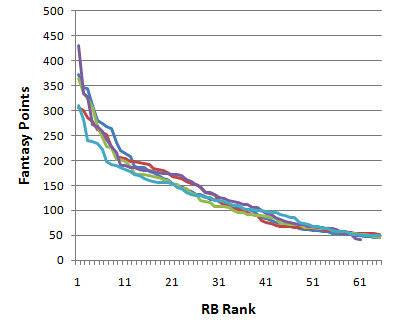
RBs are not quite as consistent from year to year as QBs, tending to retain about 48% of their previous year performance. RBs drop-off curves are not quite as steep as for the QBs, and then levels off a little quicker as evidenced in the graph below.
First tier RBs outperform 2nd tier RBs by 64 points, and the 2nd tier outperforms the 3rd tier by 31.
Wide Receivers WRs are, by far, the least consistent position, retaining only 16% of performance levels from year to year for the top 32 receivers. But because there are typically 2 primary starting WRs on each team, I also ran the correlations for the top 64 WRs each year, which would. Still, they retained only 34% of their prior year performance using this method. Either way, WR performance is the least predictable of the primary offensive positions.
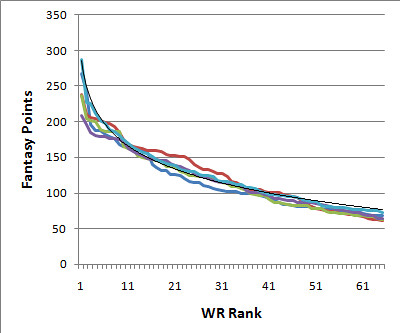
WRs are not nearly as scarce as QBs and RBs. The drop-off after the very best receivers is not as steep, and there is an abundance of mid-tier WRs deeper into the ranks.
The difference between the 1st tier WRs and the 2nd tier is 55 pts, and the difference between the 2nd and 3rd tiers is 25 pts. The differences are less than those for both QBs and RBs.
Tight Ends TE tends to be something of an afterthought in fantasy drafts. Most guys will pick up 2 RBs, a QB, and 2 or 3 WRs before grabbing a TE. They can be overlooked because as a group they don't score many fantasy points in absolute terms. But I think that's a mistake.
TEs are remarkably consistent compared to WRs. In fact, they tend to be the most consistent of all the fantasy positions. They retain 63% of their previous year's performance. The drop-off is also relatively steep.
In part 2 of this article, I'll tie together the scarcity and consistency at each position. I'll then outline a strategy that will give you a big advantage in your league's draft.
Notes:
1. Players who retired or suffered season-ending injuries in the pre-season were not included in the analysis. They would not have been in the draft, and so do not count against the consistency and scarcity measures.
2. Fantasy points were calculated using 6 pts per TD, 1 pt per 10 yds rushing, 1 pt per 25 yds passing, and -2 pts per turnover.
3. Data is from PFR and Yahoo.
The End-Game
 Late in the game, when the score is close, it's pretty obvious what the trailing team needs to do. They need to score. But what about the team ahead? Should they try to score and pad their lead? Should they pass the ball instead of running it, risking interceptions and stopping the clock? Or should they rely almost exclusively on the run, limiting risk and letting the clock run?
Combining two concepts of utility in football--expected points (EP) and win probability (WP), I'll analyze team strategy in the 4th quarter. Ultimately, we'll find out if NFL coaches are making the right strategy decisions in the end-game. If my analysis is correct, it would have meaningful implications for NFL strategy in close games.
Recap
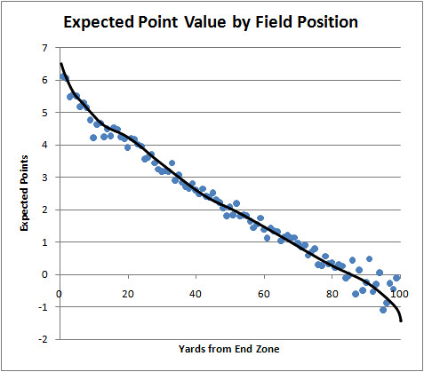
Before I get to the meat of my theory, I should review the concepts on which it's based. EP is the average number of points scored next at each field position. For example, at an opponent's 10 yd-line, a team can usually expect about 5 points on average. But on their own 10, a team would expect -0.5 points because the opponent is actually more likely to score next. For the NFL as a whole, here is what the EP curve looks like for a 1st down at each position on the field.
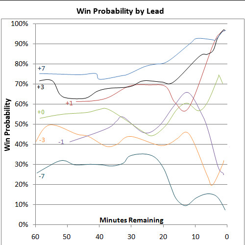
WP is the probability a team will win a game given the current score, time remaining, and any other relevant variables including field position, down and distance to go, and time outs remaining. Here is a graph of WP for selected score differentials. So far I have not made adjustments for field position or other variables, but we can already notice some very interesting things. To read the graph, each curve represents the WP of the team with the ball for a given point differential. For example, a team with the ball and a 7-point lead at halftime (30 min remaining) has a 75% chance of winning.
Observations
In the graph above, notice how the lines are somewhat steady until some point late in the 3rd quarter/early in the 4th quarter when they suddenly diverge. As time dwindles, teams with small leads become far more likely to win, and teams that are behind see their chances diminish rapidly.
Something big happens right around the 4th quarter mark that changes the nature of the game. This seems to be the point where teams stop playing a conventional contest of point maximization, and they start maneuvering for the end game. Teams that are ahead would take fewer risks while teams that are behind would take greater risks. Both teams would start managing the clock, either jockeying for that extra possession or running down the clock.
Also notice the purple line--the WP for teams with the ball and trailing by -1 point. Throughout much of the 2nd half, a team with the ball, down by 1 point, will probably win the game. I was a little surprised by that at first, but I shouldn't have been. The EP curve above shows that possession of the ball at anywhere past a team's own 30 yd-line is, on average, worth more than a point.
Effectively, this means that throughout much of the 4th quarter, teams on defense with a one point lead are already losing. They just don't know it yet.
Further, and more surprising, is the overlap in WP for teams with a +1 point lead and a -1 point deficit. In the first several minutes of the 4th quarter, a team with the ball that's down by 1 is actually more likely to win than a team with the ball and is up by 1!
What? How Can That Be?
Why would a team be better off being down by a point than ahead by a point? I think it has to do with mindset and risk tolerance. Teams that are down increase their risk tolerance and teams that are up decrease their risk tolerance. My theory is that, in general, almost all offenses usually play below the optimum risk level. They should typically be playing more aggressively. But teams may actually start to optimize when behind in the 4th quarter. Teams with small leads would restrict their risk tolerance even more, tilting further from the optimum risk-reward balance.
Consequently, teams with a very small lead need to count on the high likelihood that the opponent will score, and strategize accordingly. They should play as if they're behind, before they actually do fall behind. When the trailing team scores (and they probably will), it may be too late to become more aggressive and try to reclaim the lead.
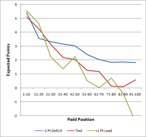
If I'm right, we should see the EP curves for teams with small leads look different from teams with small deficits. The chart below illustrates the 4th quarter EP for teams with a +1 point lead (green), tied (red), and a -1 point deficit (blue). The data set has been narrowed considerably compared to the overall NFL expected point curve, so the curves are a little noisier, but the trends are clear enough to draw conclusions.
The chart excludes the last 5 minutes of the 4th quarter. The final minutes are excluded because teams with leads of any size could simply run out the clock and leave little or no time for an opponent to score. I wanted to be sure to exclude this final possession from the analysis which would bias the results. (I'm not cherry-picking the data, as including those final minutes actually makes the differences more stark.)
There is one point at which teams with a +1 point lead become more efficient. That's inside the 20 yard line. Teams behind by a point, knowing they're within field goal range, tighten up. They effectively have a 2-point lead at this point and reduce their risk levels accordingly. Teams ahead by a point appear to keep grinding toward the end zone when inside the 20. Keeping the drive going keeps the ball out of the hands of the opponent and burns time off the clock. So the added risk of the continuing the push for the end zone may be balanced by the advantage of keeping the ball out of the opponent's hands. By this point in the game, you don't want to score too quickly. Teams that are tied even seem to be playing very timidly. Their EP profile is very similar to teams with a +1 point lead. If tied teams or teams with a lead simply played normally, or even slightly less conservatively, they'd win more often.
My advice to NFL coaches would therefore be to become more aggressive with a small lead in the 4th quarter. In fact, whatever it is teams do when down by 1 in the 4th quarter, do that all game long, even with a small lead. Go for it on 4th down more often, go no-huddle, and air it out. You'll score more and prevent your opponent from scoring more often. Ultimately, you'll win more often.
Win Probability
 Desperate for football, I'm watching the Hall of Fame Game tonight. There's four minutes left in the fourth quarter and the Redskins are up by 7 over the Colts. Can Jared Lorenzen lead his 4th-string squad to a comeback? I must be the only person in the country who cares. And I only care because I'm developing Win Probability (WP) in NFL football.
WP is simply an in-game estimate of who's going to win based on the current score and other game variables. This post will examine the potential application of WP and will illustrate a first cut at actual WP for various scores and time remaining.
Two of my recent posts discussed measures of utility in football. I looked at first down probability and at point expectancy. First down probability analyzes how likely an offense is to convert their present down and distance situation to a first down. The success of a play can be judged based on how it changes the probability of a first down. Point expectancy measures how many points a team scores on average based on its field position. This technique not only measures success, but can provide coaches with a decision-making tool. We saw, however, that both of these techniques had their limitations.
Win Probability (WP) has been a facet of baseball sabermetrics for many years. In baseball it basically measures the probability one team will win based on score, inning, outs, and runners on base. I suppose the batter's count could be included in the calculations too.
The usefulness of WP goes beyond fan curiosity about whether the home team has a chance to win (but that's interesting in itself). Take a situation in baseball with a team down by 1 run in the 9th inning. There's a runner on first base and no outs. Should the manager call for the steal? WP should instruct his decision. We could calculate the WP of the steal decision by totaling the WPs of the potential outcomes. The WP of the steal decision would be:
WP(steal) = Pr(successful steal) * WP(runner on 2nd, no outs) + Pr(caught stealing) * WP (no runners, 1 out)
This would be compared to the various outcomes of the current at bat without stealing to decide which decision gives the team the best chance to win. There would be analogous applications of WP in decision-making in football.
Baseball is a sport well-suited to WP because it has a limited number of discrete states. There are 27 outs for each team, 3 bases, and 3 outs per inning, and there is enough historical data to accurately calculate the historical WP for each state. Football is far more complex. The states are continuous and non-discrete. For example, compare field position to runners on base. There are only eight (I think) combinations of base runners, but there are 99 yard lines. Or compare each baseball team's 27 outs (54 total) to the 3600 minute and second combinations in a 60 minute football game. There is literally over a billion potential combinations of score, field position, down and distance, and time remaining.
WP in football can be simplified, thankfully. For example, time remaining can be grouped into minute or 30 second increments. Field position could be grouped in chunks too. Even so, there are still so many combinations of states in a football game that a good WP model would need a lot of data. And I'm not talking about an entire season of play-by-play information. We'd need years of data, and even then we'd need a lot of mathematical smoothing and "best fit" estimation.
The graph below is my own first cut at WP for the NFL. It is based on all regular season games from the 2000 through 2007 seasons. For the most common score differentials, it plots the WP of the team with possession of the ball. For example, the top curve, labeled +7, is the WP for a team that is winning by 7 points, and has the ball, at each minute remaining in a game. The -7 curve, at the bottom, is the WP for a team trailing by 7 points and has the ball.
It does not factor in field position or down and distance situations. So, this should be considered a baseline and not a finished product. But already we can see some interesting things.
A few things stand out to me right away. Notice the sudden drop off of the -7 curve. A team trailing by a touchdown with 20 minutes left in the game (5 min left in the 3rd quarter) sees its chance of winning fall dramatically. There are similar drop offs for teams trailing by 1 and 3 points at the beginning of the 4th quarter.
Also notice how the WP for a team down by 3 has a slight uptick, from .20 to .30, in the last few minutes of the game. I think this is because if they are able to score and at least force overtime, there is not much time left for the opponents to mount a scoring drive themselves.
One particular surprise is that teams down by 1 point early in the 4th quarter, who have the ball, are actually favored to win. By 7 minutes remaining, the team trailing by a point falls below even odds.
The application of WP could have profound consequences. Take a fairly common scenario. Your team is down by 3 points with 4 minutes left in the 4th quarter. You're facing a 4th down and goal from the 2 yard line. Conventional wisdom screams field goal! Get some points on the board and at least force OT. But WP might say something else. (Keep in mind field position is not considered yet, so this is rough).
If you kick the (virtually automatic) field goal, that ties the score and gives the opponent the ball with just less than 4 minutes remaining. Your opponent has a 70% chance of winning in this situation according to the graph. You've got a 30% chance.
Let's see what happens if you go for it. If a 4th down try for 2 yards would be successful about 30% of the time (which it is, at least for 2007), your PW is the total probability of the two outcomes:
= 0.30 * 0.92 + 0.70 * 0.22
= 0.43
 That's a 43% chance of winning by going for the TD vs. a 30% chance by going for the FG. I think this actually understates the chance of winning by going for it because if you fail, the opponent gets the ball very near his own goal line. So if you get the ball back, chances are you won't have far to go to get back into field goal range.
A lot of work still needs to be done, but the potential for WP in football is enormous.
Favre Follow-Up
 The "Brett Favre is Overrated" article has garnered a lot of attention over the past couple weeks. I enjoy reading the comments from the various message boards on which it has been linked. I'm always surprised by how many people don't trust statistics, which is probably a healthy thing. So for the few remaining doubters out there that don't buy my argument that Favre's resurgent 2007 season was primarily due an exceptionally elusive receiver corps and their copious YAC, here are some hard numbers.
In the past 2 years, the NFL gamebooks have listed the location of where each pass was thrown in six sectors--deep right, left, and middle; plus short right, left, and middle. You've probably seen the graphic during broadcasts that lists how many passes a QB has completed to various locations.
Here are Favre's completion percentages over the last two regular seasons compared to the NFL average.Pass Location NFL % Favre % Deep left 42 35 Deep middle 56 55 Deep right 42 35 Short left 67 68 Short middle 69 69 Short right 67 66 Total 63 63
Despite a very average overall completion rate, Favre's rates for deep right and deep left passes are well below average. That means in order to have an overall average completion rate, he must be gorging on the dink and dunk stuff.
I'm not the only guy with access to stats like these. Do you know who else might have them? Mike McCarthy and Ted Thompson.
Expected Points
 The previous post looked at one way of assessing the success of a football play, namely, by measuring the increase or decrease in the probability of getting a first down. We saw that, in general, an offense needs at least 5 yards on any play to break even in terms of its probability of getting a 1st down. I’ll continue the discussion by looking at another measure of utility called point expectancy.
Every spot on the field has an abstract value in terms of points. We can begin assigning values at the end zones, where having the ball has a clear and concrete value. Possessing the ball at the opponent’s end zone is worth (nearly always) 7 points. And having the ball at your own end zone is worth -2 points.
Every other yard line has a point value too. We can measure it by averaging how many points will be scored next. For example, having a 1st down and 10 from an opponent’s 20 yard line is worth, on average, about 4.2 points. Often the offense will score a touchdown, and failing that, it is likely to be able to kick a field goal. But sometimes, the offense will fail to do either, and the opponent may be the next to score. In other cases, neither team will score immediately, and they will exchange possession until someone does score. This is something I’m used to watching as a Ravens fan.
The concept of point expectancy originated with the work of Virgil Carter, a former NFL quarterback who studied operations research in the early 1970s (while an active player). Carroll, Palmer, and Thorn adapted the concept in their 1987 book The Hidden Game of Football.
One flaw in the early applications of the concept was the assumption of linearity. Both Carter and the authors of Hidden Game planted stakes for the obvious point values at both end zones and then drew a straight line between them. We’ll see that isn’t exactly right. Additionally, things change in the 4th quarter as teams with leads become conservative and teams that are behind trade overall scoring optimization for urgency.
The graph below plots the expected points for a 1st down at each yard line. For simplicity, I’ve named each yard line in terms of its distance from an opponent’s end zone. Having the ball at one’s own 20 is “the 80 yard line” for example.
One immediate application of point expectancy is measuring the cost of a turnover. If an offense loses a fumble at the 50 yard line, the expected point value swings from +2 to -2, a difference of 4 points. Or we can measure the value of a punt. If a team punts for a net 35 yards from its own 35 yard line (“the 65”), the expected point value swings from +1 to about -1, a difference of 2 points. In this regard, we could say that a turnover (at the 50) is 'twice' as bad as a punt.
Expected points is also the methodological basis of the Romer paper on kicking vs. going for a first down. In it, the author measures the expected point value of attempting a field goal or punting vs. the expected point value of ‘going for it’ on 4th down. Romer also points out that touchdowns and field goals are actually worth 1 point less than we think. Unless a score takes place with very little time remaining in a half, the other team will receive a kickoff, worth on average about 1 expected point if they have enough time remaining to mount a scoring drive. Touchdowns and field goals are not quite as valuable as thought, at least in abstract terms.
I should point out that a turnover has different values at different parts of the field. This is something researched early on at the Football Outsiders site. For example a turnover in the red zone, say at the 10, results in a swing from +5 to about +.25, for a difference of 4.75 points expected.
We can see that the neutral point on the field is at a team’s own 15 yard line. There, it’s equally likely that either team will be the next to score.
Things become more complicated when we consider other down and distance situations. Suppose at any given yard line, a pass falls incomplete on 1st and 10. Second down and 10 represents a drop off of about 0.5 points expected. Second and 9 represents a slightly smaller drop off, until at about 2nd and 5 when the expected points are approximately equal to those for 1st and 10. This is consistent with the 1st down probability method I described in my previous posts. Third down and 10 represents a further drop off of about 0.5 points. Another complication is that various teams have different curves. Defenses would each have their own curve as well. When using point expectancy to weigh decisions about kicking or going for a first down, each team would have to take into account its own and its opponent's unique expectancy curves. Take for example the Ravens and Colts over most of this decade. Each team is typical of opposing extremes--great defense, mediocre offense, and vice versa.
A drawback to this method of measuring utility in football is that it does not consider time remaining. In other words, it assumes that every game is indefinitely long and the object for each team is to maximize point differential. But this is not how football really works. Take the case of a team trailing by 4 points late in a game. A touchdown is essential, but a field goal would be pointless. Even on 4th and very long, it wouldn't make sense to purely maximize "expected" points by kicking. For the vast majority of situations in football, however, this method would be adequate. This brings me to the next method of measuring utility in football—win probability. I’ll discuss that in a forthcoming article.